GESSO Demo - Visium HD Colorectal Cancer (Tumor)
Gene set activity quantification and pathway colocalization on a sub-cellular-resolution dataset
This notebook demonstrates GESSO on the 10x Visium HD human colorectal cancer (CRC) tumor tissue at its native 541,968-spot resolution. We score the four cell-type-specific pathways highlighted in the GESSO manuscript and reproduce the manuscript’s downstream pathway colocalization analysis, which examines whether tumor-associated and epithelial-associated programs co-occur at the same locations within the tumor microenvironment.
Pathways scored (Methods, manuscript section “GESSO reveals cell-type-specific pathway activity and pathway colocalization in Visium HD human colorectal cancer data”):
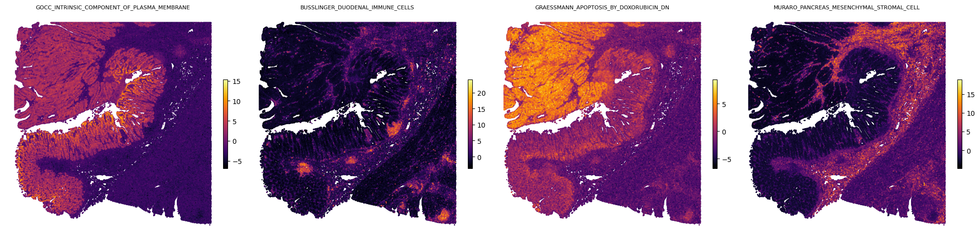
GOCC_INTRINSIC_COMPONENT_OF_PLASMA_MEMBRANE- intestinal epithelial programBUSSLINGER_DUODENAL_IMMUNE_CELLS- T-cell-associated immune programGRAESSMANN_APOPTOSIS_BY_DOXORUBICIN_DN- tumor-associated programMURARO_PANCREAS_MESENCHYMAL_STROMAL_CELL- mesenchymal stromal / fibroblast program
All paths below point to the original locations of the data on the OSCAR compute system; replace them with your own when re-running.
Import the gesso package.
The gesso Python package can be easily downloaded from source. Simply run the following script in your terminal after ensuring Python and pip are available in your environment. We recommend installing GESSO in a new Python environment.
git clone https://github.com/YMa-Lab/GESSO.git
cd gesso
pip install .
cd ..
Reading Visium HD data additionally requires scanpy (for the 10x .h5) and pyarrow (for the tissue-positions .parquet):
pip install scanpy pyarrow
[1]:
from pathlib import Path
import sys
import time
import warnings

import numpy as np
import pandas as pd
import matplotlib.pyplot as plt
import matplotlib.colors as mcolors
import scanpy as sc

warnings.filterwarnings("ignore", message="Variable names are not unique")

project_directory = Path("__notebook__").resolve().parent.parent
sys.path.append(str(project_directory))

from gesso import GESSO
Configure logging (optional)
GESSO uses Python’s standard logging module under the gesso.* hierarchy. Because the lowres method spawns one job per (gene set, partition) pair (4 × 50 = 200 jobs here), we silence the per-gene-set worker logs and only keep top-level summaries.
[2]:
from gesso import logging as glog

glog.enable()
glog.silence_per_geneset();
Load the spatial transcriptomics data.
The Visium HD output ships as a 10x .h5 count matrix (filtered_feature_bc_matrix.h5) and a tissue_positions.parquet mapping each barcode to array (row, col) coordinates. We read both, restrict to in-tissue spots, and drop spots with very low total counts (<50) as in the manuscript pipeline.
[3]:
visiumhd_root = Path(
    "/users/ayang103/data/Spatial/raw/Visium_HD/Human_CRC_FFPE/Colon_Tumor_P5/binned_outputs/square_008um"
)
expression_h5 = visiumhd_root / "filtered_feature_bc_matrix.h5"
tissue_positions_parquet = visiumhd_root / "spatial" / "tissue_positions.parquet"

pathways_csv = Path(
    "/users/ayang103/data/Project/SPLAGE/Target_Pathway_List/PathwaysTable/used_geneset"
    "/VisiumHD.CRC.PathwaysTable.0505.csv"
)
for p in (expression_h5, tissue_positions_parquet, pathways_csv):
    assert p.exists(), p
[4]:
t0 = time.time()
adata = sc.read_10x_h5(str(expression_h5))
adata.var_names_make_unique()
# expression: spots x genes (dense, float32). Visium HD count matrices are highly sparse but
# GESSO's lowres path materializes per-partition slices, so we keep a dense view.
expression_df: pd.DataFrame = pd.DataFrame(
    adata.X.toarray(), index=adata.obs_names, columns=adata.var_names
)
print(f"loaded h5 in {time.time() - t0:.1f}s; shape (spots x genes) = {expression_df.shape}")
display(expression_df.iloc[:5, :8])
loaded h5 in 25.0s; shape (spots x genes) = (541968, 18085)
| SAMD11 | NOC2L | KLHL17 | PLEKHN1 | PERM1 | HES4 | ISG15 | AGRN | |
|---|---|---|---|---|---|---|---|---|
| s_008um_00602_00290-1 | 0.0 | 0.0 | 0.0 | 0.0 | 0.0 | 0.0 | 0.0 | 0.0 |
| s_008um_00789_00234-1 | 0.0 | 0.0 | 0.0 | 0.0 | 0.0 | 0.0 | 0.0 | 0.0 |
| s_008um_00728_00006-1 | 0.0 | 0.0 | 0.0 | 0.0 | 0.0 | 0.0 | 0.0 | 0.0 |
| s_008um_00526_00291-1 | 0.0 | 0.0 | 0.0 | 0.0 | 0.0 | 0.0 | 0.0 | 0.0 |
| s_008um_00681_00396-1 | 0.0 | 0.0 | 0.0 | 0.0 | 0.0 | 0.0 | 0.0 | 0.0 |
[ ]:
locations_df = pd.read_parquet(str(tissue_positions_parquet))
locations_df = locations_df[locations_df["in_tissue"] == 1].set_index("barcode")
locations_df = locations_df.rename(columns={"array_row": "x", "array_col": "y"})[["x", "y"]]
display(locations_df.head())
print("locations shape:", locations_df.shape)

common_spots = expression_df.index.intersection(locations_df.index)
expression_df = expression_df.loc[common_spots]
locations_df = locations_df.loc[common_spots]
print("after in-tissue intersect:", expression_df.shape, locations_df.shape)

spot_total_counts = expression_df.sum(axis=1)
keep = spot_total_counts >= 50
expression_df = expression_df.loc[keep]
locations_df = locations_df.loc[keep]
print("after >=50 counts filter:", expression_df.shape, locations_df.shape)
| x | y | |
|---|---|---|
| barcode | ||
| s_008um_00000_00223-1 | 0 | 223 |
| s_008um_00000_00224-1 | 0 | 224 |
| s_008um_00000_00225-1 | 0 | 225 |
| s_008um_00000_00226-1 | 0 | 226 |
| s_008um_00000_00227-1 | 0 | 227 |
locations shape: (541968, 2)
after in-tissue intersect: (541968, 18085) (541968, 2)
after >=50 counts filter: (460894, 18085) (460894, 2)
Load the gene-set membership matrix and restrict to the four paper pathways. The pathway table is a \(G \times n_\text{genesets}\) binary matrix.
[ ]:
paper_pathways = [
    "GOCC_INTRINSIC_COMPONENT_OF_PLASMA_MEMBRANE",
    "BUSSLINGER_DUODENAL_IMMUNE_CELLS",
    "GRAESSMANN_APOPTOSIS_BY_DOXORUBICIN_DN",
    "MURARO_PANCREAS_MESENCHYMAL_STROMAL_CELL",
]

genesets_df = pd.read_csv(pathways_csv, index_col=0, usecols=["Unnamed: 0", *paper_pathways])
genesets_df = genesets_df[paper_pathways]
genesets_df.columns.name = None
genesets_df.index.name = None
for pw in paper_pathways:
    print(f"{pw}: {int(genesets_df[pw].sum())} genes")
display(genesets_df.iloc[:5])
GOCC_INTRINSIC_COMPONENT_OF_PLASMA_MEMBRANE: 1649 genes
BUSSLINGER_DUODENAL_IMMUNE_CELLS: 788 genes
GRAESSMANN_APOPTOSIS_BY_DOXORUBICIN_DN: 1670 genes
MURARO_PANCREAS_MESENCHYMAL_STROMAL_CELL: 627 genes
| GOCC_INTRINSIC_COMPONENT_OF_PLASMA_MEMBRANE | BUSSLINGER_DUODENAL_IMMUNE_CELLS | GRAESSMANN_APOPTOSIS_BY_DOXORUBICIN_DN | MURARO_PANCREAS_MESENCHYMAL_STROMAL_CELL | |
|---|---|---|---|---|
| SAMD11 | 0 | 0 | 0 | 0 |
| NOC2L | 0 | 0 | 0 | 0 |
| KLHL17 | 0 | 0 | 0 | 0 |
| PLEKHN1 | 0 | 0 | 0 | 0 |
| PERM1 | 0 | 0 | 0 | 0 |
Use GESSO to compute gene set activity scores
We use the lowres method with n_partitions=50 (~10k spots per partition) and stratified_kmeans partitioning, matching the manuscript settings. Each of the 4 gene sets is scored across all 50 spatial partitions, which the Parallel pool processes concurrently.
[7]:
model = GESSO(
    expression_df=expression_df,
    locations_df=locations_df,
    genesets_df=genesets_df,
    k=20,
    normalize_counts_method="normalize-log1p",
)

start = time.time()
gas_report = model.compute_gas(
    genesets=paper_pathways,
    beta=0.33,
    compute_method="lowres",
    partition_method="stratified_kmeans",
    n_partitions=50,
    n_jobs=40,
    store_gene_contributions=True,
)
print(f"compute_gas done in {time.time() - start:.1f} s for {len(paper_pathways)} gene sets")

gas_df = gas_report.gas_df()
display(gas_df.head())
GESSO (info): Removed 3 genes not found in geneset data. 18032 genes remain.
GESSO (info): Removed 53 genes not found in expression data. 18032 genes remain.
GESSO (info): Identified 18032 common genes in the gene set and expression data.
GESSO (info): Identified 460894 common spots in the location and expression data.
GESSO (info): Normalized expression data with strategy 'normalize-log1p'.
GESSO (info): Model initialization complete.
GESSO (info): Beginning low resolution activity score computation for 4 gene sets with 4
               jobs. Method used: lowres.
compute_gas done in 8864.0 s for 4 gene sets
| GOCC_INTRINSIC_COMPONENT_OF_PLASMA_MEMBRANE | BUSSLINGER_DUODENAL_IMMUNE_CELLS | GRAESSMANN_APOPTOSIS_BY_DOXORUBICIN_DN | MURARO_PANCREAS_MESENCHYMAL_STROMAL_CELL | |
|---|---|---|---|---|
| s_008um_00602_00290-1 | -2.952496 | -0.527955 | -2.119333 | 3.403775 |
| s_008um_00789_00234-1 | -3.144627 | -0.996569 | -1.649031 | 3.866180 |
| s_008um_00728_00006-1 | -2.745910 | 3.940566 | -1.357936 | 5.941730 |
| s_008um_00526_00291-1 | 0.331325 | -2.654313 | -2.657874 | -2.478389 |
| s_008um_00681_00396-1 | -3.018818 | -1.262808 | -1.380834 | -0.599498 |
Top gene contributions per pathway
[8]:
for pw in paper_pathways:
    top = gas_report.gene_contributions_df(geneset=pw).head(8)
    print(f"\n=== top contributors: {pw} ===")
    print(top)
=== top contributors: GOCC_INTRINSIC_COMPONENT_OF_PLASMA_MEMBRANE ===
         GOCC_INTRINSIC_COMPONENT_OF_PLASMA_MEMBRANE
CEACAM5                                     0.212709
PIGR                                        0.208471
TSPAN8                                      0.196533
MUC12                                       0.188096
SLC26A3                                     0.153996
TSPAN1                                      0.152763
CD24                                        0.137660
FXYD3                                       0.137645

=== top contributors: BUSSLINGER_DUODENAL_IMMUNE_CELLS ===
        BUSSLINGER_DUODENAL_IMMUNE_CELLS
CXCR4                           0.145287
VIM                             0.142737
SRGN                            0.135416
IL7R                            0.120010
CD52                            0.114583
LAPTM5                          0.112728
CCL5                            0.111202
IKZF1                           0.111154

=== top contributors: GRAESSMANN_APOPTOSIS_BY_DOXORUBICIN_DN ===
         GRAESSMANN_APOPTOSIS_BY_DOXORUBICIN_DN
PPDPF                                  0.118671
CD44                                   0.107779
TYMS                                   0.102382
HNF4A                                  0.100400
CYP51A1                                0.092654
RRBP1                                  0.092526
PTBP3                                  0.088923
PDHA1                                  0.087897

=== top contributors: MURARO_PANCREAS_MESENCHYMAL_STROMAL_CELL ===
        MURARO_PANCREAS_MESENCHYMAL_STROMAL_CELL
COL3A1                                  0.213950
COL1A1                                  0.199296
COL1A2                                  0.196409
MMP2                                    0.174373
VIM                                     0.171989
SPARC                                   0.158614
DCN                                     0.149974
LUM                                     0.147993
Visualize spatial maps for the four paper pathways
[9]:
fig, axes = plt.subplots(1, len(paper_pathways), figsize=(5 * len(paper_pathways), 5))
for ax, pw in zip(axes, paper_pathways):
    gas_report.plot_gas_spatial_map(
        geneset=pw, size=0.5, cmap="inferno", figsize=(5, 5), ax=ax,
    )
    ax.set_title(pw, fontsize=8)
    ax.invert_yaxis()
fig.tight_layout()
display(fig)
plt.close(fig)
Downstream: pathway colocalization in the tumor microenvironment
The manuscript reports that distinct pathway programs colocalize within tumor niches. Pairs of pathways drawn from a tumor-associated module and an epithelial-associated module exhibit increased spatial correlation in tumor tissue (Figure 5G-H). Here we reproduce that visualization on a single representative pair: the tumor-associated pathway GRAESSMANN_APOPTOSIS_BY_DOXORUBICIN_DN and the epithelial-associated pathway GOCC_INTRINSIC_COMPONENT_OF_PLASMA_MEMBRANE.
We first quantify their global colocalization with Pearson’s \(r\) across spots, then render a bivariate spatial map. Each spot is classified into one of four categories based on whether its GAS for each pathway is above or below the within-pathway median (median split per pathway): low/low, tumor-only, epithelial-only, both-high. Spots in the both-high category are the regions where the two programs colocalize.
[10]:
tumor_pw = "GRAESSMANN_APOPTOSIS_BY_DOXORUBICIN_DN"
epi_pw = "GOCC_INTRINSIC_COMPONENT_OF_PLASMA_MEMBRANE"

tumor_gas = gas_df[tumor_pw]
epi_gas = gas_df[epi_pw]

pearson_r = tumor_gas.corr(epi_gas)
print(f"Pearson r({tumor_pw}, {epi_pw}) = {pearson_r:.3f}")
Pearson r(GRAESSMANN_APOPTOSIS_BY_DOXORUBICIN_DN, GOCC_INTRINSIC_COMPONENT_OF_PLASMA_MEMBRANE) = 0.671
[ ]:
tumor_high = (tumor_gas > tumor_gas.median()).astype(int)
epi_high = (epi_gas > epi_gas.median()).astype(int)
biv_class = (2 * epi_high + tumor_high).rename("biv_class")

biv_palette = {
    0: "#dddddd",  # low/low: grey
    1: "#d7191c",  # tumor only: red
    2: "#2c7bb6",  # epithelial only: blue
    3: "#000000",  # colocalized: black
}
biv_labels = {
    0: "low / low",
    1: "tumor only",
    2: "epithelial only",
    3: "colocalized",
}

frac_coloc = (biv_class == 3).mean()
print(f"fraction of spots in 'colocalized' (both-high) category: {frac_coloc:.3f}")

plot_df = locations_df.copy()
plot_df["biv_class"] = biv_class
plot_df["color"] = plot_df["biv_class"].map(biv_palette)

fig, ax = plt.subplots(figsize=(7, 7))
ax.scatter(
    plot_df["x"], plot_df["y"],
    c=plot_df["color"], s=0.5, marker=".", linewidths=0,
)
ax.set_aspect("equal", adjustable="box")
ax.invert_yaxis()
ax.set_xticks([]); ax.set_yticks([])
for spine in ax.spines.values():
    spine.set_visible(False)
ax.set_title(
    f"Bivariate colocalization\n{tumor_pw}  \u00d7  {epi_pw}\nPearson r = {pearson_r:.3f}",
    fontsize=9,
)
handles = [plt.Line2D([0], [0], marker="o", linestyle="", color=biv_palette[i], label=biv_labels[i], markersize=8)
           for i in [0, 1, 2, 3]]
ax.legend(handles=handles, loc="lower right", fontsize=8, frameon=False)
fig.tight_layout()
display(fig)
plt.close(fig)
fraction of spots in 'colocalized' (both-high) category: 0.424
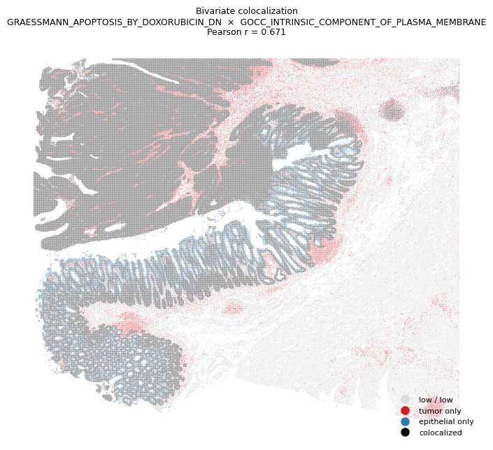
Black regions in the bivariate map correspond to spots where both the tumor-associated and epithelial-associated pathways are co-elevated. As described in the manuscript, these colocalized regions concentrate within the tumor compartment and are interpreted as coordinated tumor-epithelial cross-talk emerging during tumor progression. The same procedure can be applied to any other pathway pair drawn from the GAS table.