GESSO Demo - CosMx Human Non-Small Cell Lung Cancer Dataset
Gene set activity quantification and EMT-niche analysis on a single-molecule imaging dataset
This notebook demonstrates GESSO on the CosMx human non-small cell lung cancer (NSCLC) 3D-ECM dataset (Pentimalli et al., Cell Systems, 2025; available at Zenodo record 15240431), specifically section 22 (~58k cells). We score the five cell-type / niche pathways highlighted in the GESSO manuscript and reproduce the manuscript’s downstream EMT-niche analysis.
Pathways scored (Methods, manuscript section “GESSO resolves distinct cellular niches and EMT programs from CosMx human non-small cell lung cancer data”):
TRAVAGLINI_LUNG_ALVEOLAR_EPITHELIAL_TYPE_1_CELL- tumor coreTRAVAGLINI_LUNG_ADVENTITIAL_FIBROBLAST_CELL- desmoplastic stromaTRAVAGLINI_LUNG_PROLIFERATING_MACROPHAGE_CELL- macrophage nicheGOBP_T_CELL_ACTIVATION- T cell nicheFOROUTAN_PRODRANK_TGFB_EMT_UP- EMT niche (TGFβ-induced EMT program)
All paths below point to the original locations of the data on the OSCAR compute system. Replace them with your own when re-running.
Import the gesso package.
The gesso Python package can be easily downloaded from source. Simply run the following script in your terminal after ensuring Python and pip are available in your environment. We recommend installing GESSO in a new Python environment.
git clone https://github.com/YMa-Lab/GESSO.git
cd gesso
pip install .
cd ..
Reading CosMx .Rds files additionally requires pyreadr:
pip install pyreadr
[1]:
from pathlib import Path
import sys
import time

import numpy as np
import pandas as pd
import pyreadr
import matplotlib.pyplot as plt
import seaborn as sns
from scipy.stats import mannwhitneyu

project_directory = Path("__notebook__").resolve().parent.parent
sys.path.append(str(project_directory))

from gesso import GESSO
Configure logging (optional)
GESSO uses Python’s standard logging module under the gesso.* hierarchy. Because the lowres method spawns one job per (gene set, partition) pair (5 × 10 = 50 jobs here), we silence the per-gene-set worker logs and only keep top-level summaries.
[2]:
from gesso import logging as glog

glog.enable()
glog.silence_per_geneset();  # keep summaries, mute per-geneset progress
Load the spatial transcriptomics data.
The CosMx NSCLC data ships as R .Rds files: a count matrix (genes × cells) and a metadata table with 2-D / 3-D cell coordinates, cell-type labels, niche assignments, and an in_EMT_niche boolean column flagging cells within the manually-annotated EMT niche from the original study. We read both with pyreadr. The count matrix is transposed to (cells × genes) for GESSO.
[3]:
cosmx_data_dir = Path("/users/ayang103/data/Project/SPLAGE/ST_Data/CosMx_ECM3D")
pathways_csv = Path(
    "/users/ayang103/data/Project/SPLAGE/Target_Pathway_List/PathwaysTable/used_geneset"
    "/CosMx.NSCLC3D.PathwaysTable.0702.csv"
)

count_rds = cosmx_data_dir / "section_22_Count.Rds"
metadata_rds = cosmx_data_dir / "section_22_Metadata.Rds"
for p in (count_rds, metadata_rds, pathways_csv):
    assert p.exists(), p
[4]:
# count matrix: genes x cells, transpose to cells x genes for GESSO
t0 = time.time()
expression_df: pd.DataFrame = pyreadr.read_r(str(count_rds))[None]
expression_df.columns.name = None
expression_df.index.name = None
expression_df = expression_df.T
print(f"loaded count matrix in {time.time() - t0:.1f}s; shape (cells x genes) = {expression_df.shape}")
display(expression_df.iloc[:5, :8])
loaded count matrix in 5.2s; shape (cells x genes) = (57993, 960)
| AATK | ABL1 | ABL2 | ACE | ACE2 | ACKR1 | ACKR3 | ACKR4 | |
|---|---|---|---|---|---|---|---|---|
| section_22_fov_1_ID_1 | 0.0 | 0.0 | 0.0 | 2.0 | 0.0 | 0.0 | 0.0 | 0.0 |
| section_22_fov_1_ID_2 | 0.0 | 0.0 | 0.0 | 0.0 | 0.0 | 0.0 | 0.0 | 0.0 |
| section_22_fov_1_ID_3 | 0.0 | 0.0 | 0.0 | 0.0 | 0.0 | 0.0 | 0.0 | 0.0 |
| section_22_fov_1_ID_4 | 0.0 | 1.0 | 0.0 | 0.0 | 0.0 | 1.0 | 0.0 | 0.0 |
| section_22_fov_1_ID_5 | 0.0 | 0.0 | 0.0 | 0.0 | 2.0 | 0.0 | 0.0 | 0.0 |
[ ]:
metadata_df: pd.DataFrame = pyreadr.read_r(str(metadata_rds))[None]
metadata_df.columns.name = None
metadata_df.index.name = None
print("metadata shape:", metadata_df.shape)
display(metadata_df[["x_2D_px", "y_2D_px", "celltypes", "niches_2D", "in_EMT_niche"]].head())
metadata shape: (57993, 63)
| x_2D_px | y_2D_px | celltypes | niches_2D | in_EMT_niche | |
|---|---|---|---|---|---|
| section_22_fov_1_ID_1 | 21290.0 | 3613.0 | Vascular endothelium | Vascular stroma | False |
| section_22_fov_1_ID_2 | 20855.0 | 3619.0 | Regulatory T cells | T cell niches | False |
| section_22_fov_1_ID_3 | 19758.0 | 3607.0 | Tumor cells | Tumor core | False |
| section_22_fov_1_ID_4 | 19584.0 | 3584.0 | Tumor cells | Tumor core | False |
| section_22_fov_1_ID_5 | 19465.0 | 3619.0 | Basal epithelial cells | Tumor core | False |
Filter cells to those with at least 50 total counts and align expression rows with the metadata index.
[ ]:
# >=50 total counts
spot_total_counts = expression_df.sum(axis=1)
keep_counts = spot_total_counts >= 50
print(f"cells passing >=50 counts: {int(keep_counts.sum())} / {len(keep_counts)}")

expression_df = expression_df.loc[keep_counts]

# align with metadata on cell IDs
common_cells = expression_df.index.intersection(metadata_df.index)
expression_df = expression_df.loc[common_cells]
metadata_df = metadata_df.loc[common_cells]

# GESSO locations dataframe
locations_df = metadata_df[["x_2D_px", "y_2D_px"]].rename(
    columns={"x_2D_px": "x", "y_2D_px": "y"}
).astype(float)

print("expression shape (cells x genes):", expression_df.shape)
print("locations shape:", locations_df.shape)
display(locations_df.head())
cells passing >=50 counts: 57993 / 57993
expression shape (cells x genes): (57993, 960)
locations shape: (57993, 2)
| x | y | |
|---|---|---|
| section_22_fov_1_ID_1 | 21290.0 | 3613.0 |
| section_22_fov_1_ID_2 | 20855.0 | 3619.0 |
| section_22_fov_1_ID_3 | 19758.0 | 3607.0 |
| section_22_fov_1_ID_4 | 19584.0 | 3584.0 |
| section_22_fov_1_ID_5 | 19465.0 | 3619.0 |
Load the gene-set membership matrix, restricting to five pathways. The pathway table is a \(G \times n_\text{genesets}\) binary matrix.
[ ]:
paper_pathways = [
    "TRAVAGLINI_LUNG_ALVEOLAR_EPITHELIAL_TYPE_1_CELL",
    "TRAVAGLINI_LUNG_ADVENTITIAL_FIBROBLAST_CELL",
    "TRAVAGLINI_LUNG_PROLIFERATING_MACROPHAGE_CELL",
    "GOBP_T_CELL_ACTIVATION",
    "FOROUTAN_PRODRANK_TGFB_EMT_UP",
]
genesets_df = pd.read_csv(
    pathways_csv, index_col=0, usecols=["Unnamed: 0", *paper_pathways]
)
genesets_df = genesets_df[paper_pathways]  # column order
genesets_df.columns.name = None
genesets_df.index.name = None
for pw in paper_pathways:
    print(f"{pw}: {int(genesets_df[pw].sum())} genes in CosMx panel")
display(genesets_df.iloc[:5])
TRAVAGLINI_LUNG_ALVEOLAR_EPITHELIAL_TYPE_1_CELL: 65 genes in CosMx panel
TRAVAGLINI_LUNG_ADVENTITIAL_FIBROBLAST_CELL: 75 genes in CosMx panel
TRAVAGLINI_LUNG_PROLIFERATING_MACROPHAGE_CELL: 124 genes in CosMx panel
GOBP_T_CELL_ACTIVATION: 163 genes in CosMx panel
FOROUTAN_PRODRANK_TGFB_EMT_UP: 47 genes in CosMx panel
| TRAVAGLINI_LUNG_ALVEOLAR_EPITHELIAL_TYPE_1_CELL | TRAVAGLINI_LUNG_ADVENTITIAL_FIBROBLAST_CELL | TRAVAGLINI_LUNG_PROLIFERATING_MACROPHAGE_CELL | GOBP_T_CELL_ACTIVATION | FOROUTAN_PRODRANK_TGFB_EMT_UP | |
|---|---|---|---|---|---|
| AATK | 0 | 0 | 0 | 0 | 0 |
| ABL1 | 0 | 1 | 0 | 1 | 0 |
| ABL2 | 0 | 1 | 0 | 1 | 0 |
| ACE | 0 | 0 | 0 | 0 | 0 |
| ACE2 | 0 | 0 | 0 | 0 | 0 |
Use GESSO to compute gene set activity scores
For ~55k cells we use the lowres method with n_partitions=10 (~5,500 cells per partition) and stratified_kmeans partitioning. Each of the 5 gene sets is scored across all 10 spatial partitions, which the Parallel pool processes concurrently.
[ ]:
model = GESSO(
    expression_df=expression_df,
    locations_df=locations_df,
    genesets_df=genesets_df,
    k=20,                                 # number of nearest-neighbor edges for the spatial graph
    normalize_counts_method="normalize-log1p",
)

start = time.time()
gas_report = model.compute_gas(
    genesets=paper_pathways,
    beta=0.33,                            # spatial smoothing strength
    compute_method="lowres",              # scalable estimator for high-resolution data
    partition_method="stratified_kmeans",
    n_partitions=10,
    n_jobs=20,
    store_gene_contributions=True,
)
print(f"compute_gas done in {time.time() - start:.1f} s for {len(paper_pathways)} gene sets")

gas_df = gas_report.gas_df()
display(gas_df.head())
GESSO (info): Identified 960 common genes in the gene set and expression data.
GESSO (info): Identified 57993 common spots in the location and expression data.
GESSO (info): Normalized expression data with strategy 'normalize-log1p'.
GESSO (info): Model initialization complete.
GESSO (info): Beginning low resolution activity score computation for 5 gene sets with 5
               jobs. Method used: lowres.
compute_gas done in 99.7 s for 5 gene sets
| TRAVAGLINI_LUNG_ALVEOLAR_EPITHELIAL_TYPE_1_CELL | TRAVAGLINI_LUNG_ADVENTITIAL_FIBROBLAST_CELL | TRAVAGLINI_LUNG_PROLIFERATING_MACROPHAGE_CELL | GOBP_T_CELL_ACTIVATION | FOROUTAN_PRODRANK_TGFB_EMT_UP | |
|---|---|---|---|---|---|
| section_22_fov_1_ID_1 | -2.699694 | -1.645662 | 0.174056 | -1.023556 | 0.771783 |
| section_22_fov_1_ID_2 | -1.747796 | -0.850772 | 1.699003 | 1.707946 | -1.099110 |
| section_22_fov_1_ID_3 | 3.387635 | -2.468578 | -2.451914 | -0.724324 | -0.944858 |
| section_22_fov_1_ID_4 | 5.418164 | -2.737936 | -2.478748 | -1.364351 | -2.103028 |
| section_22_fov_1_ID_5 | 0.618019 | 0.024656 | -0.645437 | -1.406777 | -1.199882 |
Top gene contributions per pathway recover well-established marker genes: epithelial / tumorigenic genes for the alveolar-type-1 program (e.g. CLDN4, EPCAM, KRT19), collagen / matrix genes for the adventitial fibroblast program (COL1A1, COL3A1), and fibroblast / mesenchymal / matrix-remodeling genes for the TGFβ-EMT program (COL1A1, COL5A1, FN1, MMP2).
[9]:
for pw in paper_pathways:
    top = gas_report.gene_contributions_df(geneset=pw).head(8)
    print(f"\n=== top contributors: {pw} ===")
    print(top)
=== top contributors: TRAVAGLINI_LUNG_ALVEOLAR_EPITHELIAL_TYPE_1_CELL ===
         TRAVAGLINI_LUNG_ALVEOLAR_EPITHELIAL_TYPE_1_CELL
CLDN4                                           0.284582
ITGA3                                           0.275478
EPCAM                                           0.271797
KRT19                                           0.264341
VEGFA                                           0.258548
S100A10                                         0.258174
KRT7                                            0.225759
TM4SF1                                          0.221621

=== top contributors: TRAVAGLINI_LUNG_ADVENTITIAL_FIBROBLAST_CELL ===
        TRAVAGLINI_LUNG_ADVENTITIAL_FIBROBLAST_CELL
COL3A1                                     0.312670
COL1A2                                     0.307957
COL1A1                                     0.280837
COL6A3                                     0.259313
LUM                                        0.253207
DCN                                        0.235834
MMP2                                       0.229944
THBS2                                      0.225030

=== top contributors: TRAVAGLINI_LUNG_PROLIFERATING_MACROPHAGE_CELL ===
        TRAVAGLINI_LUNG_PROLIFERATING_MACROPHAGE_CELL
CD68                                         0.245187
C1QB                                         0.235716
C1QA                                         0.235062
LYZ                                          0.228164
C1QC                                         0.216709
FCGR3A                                       0.209848
FCER1G                                       0.171671
MRC1                                         0.170195

=== top contributors: GOBP_T_CELL_ACTIVATION ===
       GOBP_T_CELL_ACTIVATION
CD2                  0.255129
CCL5                 0.225278
PTPRC                0.212599
IL2RG                0.211040
ITGAL                0.199418
CD3E                 0.195569
CD8A                 0.172270
CD3G                 0.147654

=== top contributors: FOROUTAN_PRODRANK_TGFB_EMT_UP ===
        FOROUTAN_PRODRANK_TGFB_EMT_UP
COL1A1                       0.358375
FN1                          0.310828
MMP2                         0.295498
COL5A1                       0.292040
CALD1                        0.253238
TAGLN                        0.248496
VCAN                         0.239680
CDH11                        0.215985
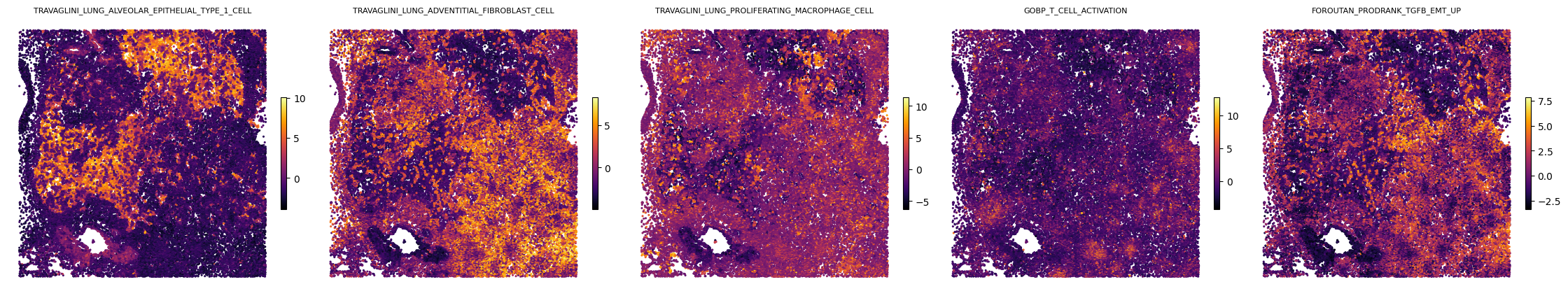
Visualize spatial maps for the five paper pathways
Per-cell GAS plotted on CosMx 2-D pixel coordinates (x_2D_px, y_2D_px). The y-axis is inverted to match anatomical orientation.
[10]:
fig, axes = plt.subplots(1, len(paper_pathways), figsize=(4.5 * len(paper_pathways), 4.5))
for ax, pw in zip(axes, paper_pathways):
    gas_report.plot_gas_spatial_map(
        geneset=pw, size=1.5, cmap="inferno", figsize=(4.5, 4.5), ax=ax,
    )
    ax.set_aspect("equal", adjustable="box")
    ax.invert_yaxis()
    ax.set_title(pw, fontsize=8)
fig.tight_layout()
display(fig)
plt.close(fig)
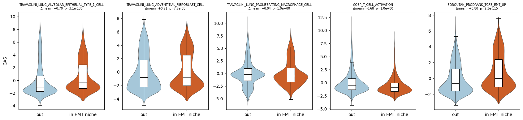
Downstream: EMT-niche enrichment
In the manuscript, we identified an EMT niche between the tumor core and the desmoplastic stroma (Figure 7E). The metadata column in_EMT_niche (boolean) marks the ~4,000 cells inside this niche. The GAS for the TGFβ-induced EMT pathway FOROUTAN_PRODRANK_TGFB_EMT_UP is strongly elevated specifically within this niche (Figure 7F).
We assess this two ways:
Distribution split: violin/boxplot of each pathway’s GAS for in-niche vs. out-of-niche cells.
Spatial overlay: the EMT GAS map alongside the niche mask, so that the agreement is visible by eye.
We also report a one-sided Mann-Whitney \(U\) test for EMT GAS in-niche > EMT GAS out-of-niche.
[11]:
emt_pw = "FOROUTAN_PRODRANK_TGFB_EMT_UP"

in_niche = metadata_df["in_EMT_niche"].astype(bool).to_numpy()
print(f"cells in EMT niche: {int(in_niche.sum())}  /  out: {int((~in_niche).sum())}")

# numeric summary across all 5 pathways, with formal test on the EMT pathway
summary_rows = []
for pw in paper_pathways:
    values = gas_df[pw].to_numpy()
    inside = values[in_niche]
    outside = values[~in_niche]
    u_stat, p_one_sided = mannwhitneyu(inside, outside, alternative="greater")
    summary_rows.append({
        "pathway": pw,
        "mean_in_niche": float(inside.mean()),
        "mean_out_niche": float(outside.mean()),
        "delta_mean": float(inside.mean() - outside.mean()),
        "mwu_pvalue_in_gt_out": float(p_one_sided),
    })

summary_df = pd.DataFrame(summary_rows).set_index("pathway")
display(summary_df)
print(f"\nMann-Whitney U (one-sided, in-niche > out-of-niche) for {emt_pw}:")
print(f"  p = {summary_df.loc[emt_pw, 'mwu_pvalue_in_gt_out']:.2e}")
print(f"  delta(mean GAS) = {summary_df.loc[emt_pw, 'delta_mean']:.3f}")
cells in EMT niche: 4082 / out: 53911
| mean_in_niche | mean_out_niche | delta_mean | mwu_pvalue_in_gt_out | |
|---|---|---|---|---|
| pathway | ||||
| TRAVAGLINI_LUNG_ALVEOLAR_EPITHELIAL_TYPE_1_CELL | 0.645455 | -0.050107 | 0.695562 | 3.088954e-130 |
| TRAVAGLINI_LUNG_ADVENTITIAL_FIBROBLAST_CELL | 0.179579 | -0.031555 | 0.211135 | 7.659245e-08 |
| TRAVAGLINI_LUNG_PROLIFERATING_MACROPHAGE_CELL | 0.042903 | 0.003655 | 0.039248 | 9.999169e-01 |
| GOBP_T_CELL_ACTIVATION | -0.615222 | 0.067794 | -0.683016 | 1.000000e+00 |
| FOROUTAN_PRODRANK_TGFB_EMT_UP | 0.728262 | -0.070010 | 0.798272 | 2.348064e-115 |
Mann-Whitney U (one-sided, in-niche > out-of-niche) for FOROUTAN_PRODRANK_TGFB_EMT_UP:
  p = 2.35e-115
  delta(mean GAS) = 0.798
[12]:
# violin + box of GAS distribution split by in_EMT_niche, one panel per pathway
niche_labels = np.where(in_niche, "in EMT niche", "out")
plot_records = []
for pw in paper_pathways:
    plot_records.append(pd.DataFrame({
        "pathway": pw,
        "GAS": gas_df[pw].to_numpy(),
        "niche": niche_labels,
    }))
plot_df = pd.concat(plot_records, ignore_index=True)

fig, axes = plt.subplots(1, len(paper_pathways), figsize=(3.4 * len(paper_pathways), 4), sharey=False)
order = ["out", "in EMT niche"]
palette = {"out": "#9ecae1", "in EMT niche": "#e6550d"}
for ax, pw in zip(axes, paper_pathways):
    sub = plot_df[plot_df["pathway"] == pw]
    sns.violinplot(
        data=sub, x="niche", y="GAS", order=order, palette=palette,
        inner=None, cut=0, linewidth=0.6, ax=ax,
    )
    sns.boxplot(
        data=sub, x="niche", y="GAS", order=order,
        width=0.18, showfliers=False, ax=ax,
        boxprops={"facecolor": "white", "edgecolor": "black", "linewidth": 0.8},
        medianprops={"color": "black", "linewidth": 1.2},
        whiskerprops={"color": "black", "linewidth": 0.8},
        capprops={"color": "black", "linewidth": 0.8},
    )
    delta = summary_df.loc[pw, "delta_mean"]
    pval = summary_df.loc[pw, "mwu_pvalue_in_gt_out"]
    ax.set_title(f"{pw}\ndelta_mean={delta:+.2f}  p={pval:.1e}", fontsize=7)
    ax.set_xlabel("")
    ax.set_ylabel("GAS" if ax is axes[0] else "")
fig.tight_layout()
display(fig)
plt.close(fig)
/tmp/ipykernel_155033/1888786270.py:17: FutureWarning:

Passing `palette` without assigning `hue` is deprecated and will be removed in v0.14.0. Assign the `x` variable to `hue` and set `legend=False` for the same effect.

  sns.violinplot(
/tmp/ipykernel_155033/1888786270.py:17: FutureWarning:

Passing `palette` without assigning `hue` is deprecated and will be removed in v0.14.0. Assign the `x` variable to `hue` and set `legend=False` for the same effect.

  sns.violinplot(
/tmp/ipykernel_155033/1888786270.py:17: FutureWarning:

Passing `palette` without assigning `hue` is deprecated and will be removed in v0.14.0. Assign the `x` variable to `hue` and set `legend=False` for the same effect.

  sns.violinplot(
/tmp/ipykernel_155033/1888786270.py:17: FutureWarning:

Passing `palette` without assigning `hue` is deprecated and will be removed in v0.14.0. Assign the `x` variable to `hue` and set `legend=False` for the same effect.

  sns.violinplot(
/tmp/ipykernel_155033/1888786270.py:17: FutureWarning:

Passing `palette` without assigning `hue` is deprecated and will be removed in v0.14.0. Assign the `x` variable to `hue` and set `legend=False` for the same effect.

  sns.violinplot(
[13]:
# spatial overlay: EMT GAS heatmap (left) vs. niche mask (right) on the same coordinates
emt_values = gas_df[emt_pw].to_numpy()
coords = locations_df[["x", "y"]].to_numpy()

fig, axes = plt.subplots(1, 2, figsize=(11, 5.5))

# left: EMT GAS heatmap
vmin = float(np.percentile(emt_values, 1))
vmax = float(np.percentile(emt_values, 99))
sc0 = axes[0].scatter(
    coords[:, 0], coords[:, 1], c=emt_values, cmap="inferno",
    s=1.5, marker=".", linewidths=0, vmin=vmin, vmax=vmax,
)
axes[0].set_aspect("equal", adjustable="box")
axes[0].invert_yaxis()
axes[0].set_xticks([]); axes[0].set_yticks([])
for spine in axes[0].spines.values():
    spine.set_visible(False)
axes[0].set_title(f"{emt_pw}\nGESSO GAS", fontsize=8)
cbar = fig.colorbar(sc0, ax=axes[0], shrink=0.7)
cbar.set_label("GAS", fontsize=8)

# right: niche mask. out-of-niche grey, in-niche red
mask_color = np.where(in_niche, "#d7191c", "#dddddd")
order = np.argsort(in_niche.astype(int))  # draw in-niche on top
axes[1].scatter(
    coords[order, 0], coords[order, 1], c=mask_color[order],
    s=1.5, marker=".", linewidths=0,
)
axes[1].set_aspect("equal", adjustable="box")
axes[1].invert_yaxis()
axes[1].set_xticks([]); axes[1].set_yticks([])
for spine in axes[1].spines.values():
    spine.set_visible(False)
axes[1].set_title("EMT niche mask\n(red = in_EMT_niche)", fontsize=8)
legend_handles = [
    plt.Line2D([0], [0], marker="o", linestyle="", color="#d7191c", label="in EMT niche", markersize=7),
    plt.Line2D([0], [0], marker="o", linestyle="", color="#dddddd", label="out", markersize=7),
]
axes[1].legend(handles=legend_handles, loc="lower right", fontsize=7, frameon=False)

fig.tight_layout()
display(fig)
plt.close(fig)
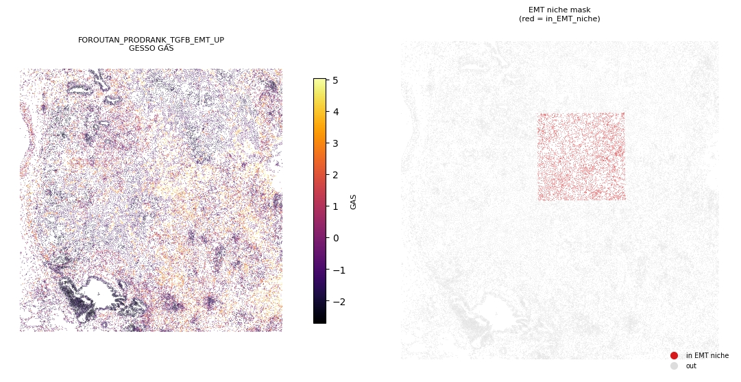
The boxplot panels show that the TGFβ-EMT pathway GAS is sharply elevated in cells inside in_EMT_niche relative to those outside, while the other niche-specific pathways shift much less in that contrast. The spatial overlay confirms this visually as the inferno-colored high-GAS region in the EMT pathway map coincides with the red niche mask. This recapitulates the manuscript’s Figure 7E-F finding that GESSO localizes EMT activity to the manually-annotated EMT niche at the tumor-stroma
interface.