GESSO Demo - 10x Visium BRCA Dataset
Gene set expression quantification with GESSO
GESSO (Gene sEt activity Score analysis with Spatial lOcation) is a computational method for quantifying the overall expression levels of gene sets for spatial transcriptomics data.
Given spatial transcriptomics data and a user-provided gene set, GESSO returns a gene set activity score (GAS) for each spot. GESSO can also systematically identify spots with elevated gene set activity through a permutation-based hypothesis test.
This notebook provides an overview of GESSO on a small dataset (a subset of human tumor 10x Visium BRCA from https://www.10xgenomics.com/datasets). This small dataset can be immediately downloaded from https://github.com/YMa-lab/GESSO/tree/main/demo_data.
Import the gesso package.
The gesso Python package can be easily downloaded from source. Simply run the following script in your terminal after ensuring Python and pip are available in your environment. We recommend installing GESSO in a new Python environment.
git clone https://github.com/YMa-Lab/GESSO.git
cd gesso
pip install .
cd ..
[1]:
from pathlib import Path
import pandas as pd
import sys

project_directory = Path("__notebook__").resolve().parent.parent
sys.path.append(str(project_directory))

from gesso import GESSO
Configure logging (optional)
GESSO uses Python’s standard logging module under the gesso.* hierarchy. By default the package is silent. Use the gesso.logging submodule to turn on console output, attach a log file, or silence the chatty per-geneset progress messages. You can also just call print(...) from your own code as usual - GESSO’s logging is independent of standard print.
Common patterns:
from gesso import logging as glog

glog.enable()                  # print INFO messages to stderr
glog.set_level("DEBUG")        # show debug-level messages
glog.silence_per_geneset()     # mute per-geneset progress, keep summaries
glog.unsilence_per_geneset()   # re-enable per-geneset progress
h = glog.add_file_handler("gesso.log", level="DEBUG")  # also log to a file
glog.remove_handler(h)         # detach when done
glog.disable()                 # back to silent
Sub-loggers gesso.init, gesso.compute, and gesso.compute.geneset can be configured independently via glog.set_level(level, logger=...) if you want even finer control.
[2]:
from gesso import logging as glog

# enable console logging at INFO level for the rest of the notebook
glog.enable();
Load the spatial transcriptomics data.
In this demo, we’ll analyze the 10x Visium BRCA dataset. Let’s first load and inspect the gene expression count data. The gene expression dataframe should be of dimension \(N \times G\), where \(N\) denotes the number of spots, and \(G\) denotes the number of genes.
[3]:
expression_df: pd.DataFrame = pd.read_pickle(
    project_directory / "demo_data" / "10xVisiumBRCA-count_data.pkl"
)
display(expression_df.head())
| gene | DVL1 | PIK3CD | MTOR | CASP9 | WNT4 | E2F2 | HDAC1 | CSF3R | SLC2A1 | PTCH2 | ... | TLR8 | VEGFD | ARAF | AR | IL2RG | FGF16 | COL4A6 | XIAP | FGF13 | IKBKG |
|---|---|---|---|---|---|---|---|---|---|---|---|---|---|---|---|---|---|---|---|---|---|
| barcode | |||||||||||||||||||||
| GTAGACAACCGATGAA-1 | 0.0 | 0.0 | 2.0 | 0.0 | 0.0 | 0.0 | 0.0 | 1.0 | 0.0 | 0.0 | ... | 0.0 | 1.0 | 1.0 | 0.0 | 3.0 | 0.0 | 0.0 | 0.0 | 0.0 | 0.0 |
| ACAGATTAGGTTAGTG-1 | 0.0 | 1.0 | 0.0 | 0.0 | 0.0 | 0.0 | 0.0 | 2.0 | 0.0 | 0.0 | ... | 0.0 | 0.0 | 1.0 | 1.0 | 1.0 | 0.0 | 0.0 | 0.0 | 0.0 | 0.0 |
| TGGTATCGGTCTGTAT-1 | 1.0 | 0.0 | 0.0 | 0.0 | 0.0 | 0.0 | 0.0 | 0.0 | 0.0 | 0.0 | ... | 0.0 | 0.0 | 0.0 | 0.0 | 0.0 | 0.0 | 0.0 | 0.0 | 1.0 | 0.0 |
| ATTATCTCGACAGATC-1 | 0.0 | 0.0 | 0.0 | 0.0 | 0.0 | 0.0 | 0.0 | 1.0 | 0.0 | 0.0 | ... | 0.0 | 0.0 | 0.0 | 0.0 | 0.0 | 0.0 | 0.0 | 0.0 | 2.0 | 0.0 |
| TGAGATCAAATACTCA-1 | 1.0 | 0.0 | 1.0 | 0.0 | 0.0 | 0.0 | 0.0 | 1.0 | 0.0 | 0.0 | ... | 0.0 | 0.0 | 1.0 | 0.0 | 0.0 | 0.0 | 0.0 | 1.0 | 0.0 | 0.0 |
5 rows × 334 columns
Next, let’s load and inspect the spatial location data. The location data is of dimension \(N \times 2\). Note: the index of the location dataframe must match the columns of the expression dataframe.
[4]:
locations_df: pd.DataFrame = pd.read_pickle(
    project_directory / "demo_data" / "10xVisiumBRCA-location_data.pkl"
)
display(locations_df.head())

# note: GESSO requires spatial locations to be in the form of a DataFrame containing columns "x" and "y"
locations_df = locations_df.rename(columns={"array_row": "x", "array_col": "y"})
display(locations_df.head())
| array_row | array_col | |
|---|---|---|
| barcode | ||
| GTAGACAACCGATGAA-1 | 7 | 55 |
| ACAGATTAGGTTAGTG-1 | 7 | 57 |
| TGGTATCGGTCTGTAT-1 | 7 | 59 |
| ATTATCTCGACAGATC-1 | 7 | 61 |
| TGAGATCAAATACTCA-1 | 7 | 63 |
| x | y | |
|---|---|---|
| barcode | ||
| GTAGACAACCGATGAA-1 | 7 | 55 |
| ACAGATTAGGTTAGTG-1 | 7 | 57 |
| TGGTATCGGTCTGTAT-1 | 7 | 59 |
| ATTATCTCGACAGATC-1 | 7 | 61 |
| TGAGATCAAATACTCA-1 | 7 | 63 |
Finally, let’s load the gene set/pathway data. This data may be stored as a \(G \times n_\text{genesets}\) binary matrix.
[5]:
genesets_df: pd.DataFrame = pd.read_pickle(
    project_directory / "demo_data" / "10xVisiumBRCA-pathways_data.pkl"
)
display(genesets_df.head())

# we can also work with gene sets as dictionaries mapping gene set name to list of genes
genesets_dict = {
    geneset: list(genesets_df.index[genesets_df[geneset] == 1])
    for geneset in genesets_df.columns
}
print(genesets_dict)
| KEGG_PATHWAYS_IN_CANCER | WP_INTERACTIONS_BETWEEN_IMMUNE_CELLS_AND_MICRORNAS_IN_TUMOR_MICROENVIRONMENT | |
|---|---|---|
| DVL1 | 1 | 0 |
| PIK3CD | 1 | 0 |
| MTOR | 1 | 0 |
| CASP9 | 1 | 0 |
| WNT4 | 1 | 0 |
{'KEGG_PATHWAYS_IN_CANCER': ['DVL1', 'PIK3CD', 'MTOR', 'CASP9', 'WNT4', 'E2F2', 'HDAC1', 'CSF3R', 'SLC2A1', 'PTCH2', 'PIK3R3', 'JUN', 'JAK1', 'WNT2B', 'NRAS', 'PIAS3', 'ARNT', 'NTRK1', 'RXRG', 'FASLG', 'LAMC1', 'LAMC2', 'TPR', 'PTGS2', 'RASSF5', 'LAMB3', 'TRAF5', 'TGFB2', 'WNT9A', 'WNT3A', 'EGLN1', 'FH', 'AKT3', 'SOS1', 'EPAS1', 'MSH2', 'MSH6', 'TGFA', 'CTNNA2', 'TCF7L1', 'PAX8', 'RALB', 'GLI2', 'ITGA6', 'ITGAV', 'STAT1', 'CASP8', 'FZD7', 'FZD5', 'FN1', 'STK36', 'WNT6', 'WNT10A', 'COL4A4', 'VHL', 'PPARG', 'RAF1', 'WNT7A', 'RARB', 'TGFBR2', 'MLH1', 'CTNNB1', 'LAMB2', 'RHOA', 'RASSF1', 'WNT5A', 'APPL1', 'MITF', 'TFG', 'CBLB', 'GSK3B', 'PIK3CB', 'MECOM', 'PLD1', 'PIK3CA', 'DVL3', 'FGF12', 'CTBP1', 'FGFR3', 'PDGFRA', 'KIT', 'CXCL8', 'FGF5', 'MAPK10', 'NFKB1', 'LEF1', 'EGF', 'FGF2', 'HHIP', 'VEGFC', 'CASP3', 'SKP2', 'FGF10', 'ITGA2', 'PIK3R1', 'MSH3', 'APC', 'TCF7', 'WNT8A', 'CTNNA1', 'FGF1', 'CSF1R', 'PDGFRB', 'FGF18', 'MAPK9', 'E2F3', 'RXRB', 'PPARD', 'CDKN1A', 'VEGFA', 'HSP90AB1', 'LAMA4', 'HDAC2', 'LAMA2', 'PDGFA', 'RAC1', 'IL6', 'CYCS', 'RALA', 'GLI3', 'EGFR', 'FZD9', 'HGF', 'FZD1', 'CDK6', 'PIK3CG', 'LAMB1', 'LAMB4', 'MET', 'WNT2', 'WNT16', 'SMO', 'BRAF', 'SHH', 'FGF20', 'FGF17', 'NKX3-1', 'FZD3', 'FGFR1', 'IKBKB', 'CCNE2', 'FZD6', 'MYC', 'PTK2', 'CDKN2B', 'DAPK1', 'PTCH1', 'TGFBR1', 'TRAF1', 'ABL1', 'LAMC3', 'RALGDS', 'RXRA', 'TRAF2', 'ITGB1', 'CUL2', 'FZD8', 'RET', 'NCOA4', 'MAPK8', 'CCDC6', 'CTNNA3', 'PTEN', 'FAS', 'CHUK', 'WNT8B', 'FGF8', 'NFKB2', 'SUFU', 'TCF7L2', 'FGFR2', 'HRAS', 'TRAF6', 'SPI1', 'VEGFB', 'BAD', 'RELA', 'GSTP1', 'CCND1', 'FGF19', 'FGF4', 'FGF3', 'FADD', 'WNT11', 'FZD4', 'BIRC3', 'BIRC2', 'MMP1', 'ZBTB16', 'CBL', 'ETS1', 'WNT5B', 'FGF23', 'FGF6', 'CDKN1B', 'KRAS', 'WNT10B', 'WNT1', 'CDK2', 'GLI1', 'CDK4', 'MDM2', 'KITLG', 'IGF1', 'HSP90B1', 'FGF9', 'FLT3', 'BRCA2', 'CCNA1', 'FOXO1', 'RB1', 'FGF14', 'COL4A1', 'COL4A2', 'EGLN3', 'NFKBIA', 'SOS2', 'BMP4', 'HIF1A', 'MAX', 'PGF', 'FOS', 'TGFB3', 'HSP90AA1', 'TRAF3', 'AKT1', 'RAD51', 'FGF7', 'DAPK2', 'MAP2K1', 'SMAD3', 'PIAS1', 'PML', 'ARNT2', 'IGF1R', 'AXIN1', 'CREBBP', 'PRKCB', 'MAPK3', 'MMP2', 'CDH1', 'PLCG2', 'CRK', 'DVL2', 'FGF11', 'TP53', 'PIK3R5', 'NOS2', 'TRAF4', 'ERBB2', 'RARA', 'JUP', 'STAT5B', 'STAT5A', 'STAT3', 'ITGA2B', 'FZD2', 'WNT3', 'WNT9B', 'ITGA3', 'AXIN2', 'PRKCA', 'GRB2', 'BIRC5', 'LAMA1', 'RALBP1', 'LAMA3', 'PIAS2', 'SMAD2', 'SMAD4', 'DCC', 'BCL2', 'FGF22', 'APC2', 'DAPK3', 'PIAS4', 'MAP2K2', 'PIK3R2', 'CCNE1', 'CEBPA', 'AKT2', 'EGLN2', 'TGFB1', 'CBLC', 'FGF21', 'BAX', 'FLT3LG', 'KLK3', 'PRKCG', 'BMP2', 'BCL2L1', 'E2F1', 'PLCG1', 'STK4', 'MMP9', 'LAMA5', 'RUNX1', 'BID', 'CRKL', 'MAPK1', 'BCR', 'RAC2', 'PDGFB', 'RBX1', 'EP300', 'WNT7B', 'CSF2RA', 'VEGFD', 'ARAF', 'AR', 'FGF16', 'COL4A6', 'XIAP', 'FGF13', 'IKBKG'], 'WP_INTERACTIONS_BETWEEN_IMMUNE_CELLS_AND_MICRORNAS_IN_TUMOR_MICROENVIRONMENT': ['PIAS3', 'TGFB2', 'CTLA4', 'PDCD1', 'TGFBR2', 'CD80', 'CD86', 'CXCL10', 'NFKB1', 'IL4', 'CD274', 'TLR4', 'IL2RA', 'NFKB2', 'TRAF6', 'IRAK4', 'STAT6', 'TGFB3', 'SOCS1', 'IL4R', 'CCL2', 'CCL5', 'STAT3', 'TGFB1', 'IL2RB', 'TLR7', 'TLR8', 'IL2RG']}
Use GESSO to compute gene set activity scores
This is the simplest use case for GESSO. Simply inpute the data and generate an activity scores report.
[6]:
model = GESSO(
expression_df=expression_df,
locations_df=locations_df,
genesets_df=genesets_df,
k=6, # increase k to increase spatial smoothing effect
normalize_counts_method="normalize-log1p", # easily normalize counts for non-preprocessed data
)
# compute activity scores for all gene sets in genesets_df
gas_report = model.compute_gas(
beta=0.33, # increase beta to increase spatial smoothing strength; must be between 0 and 1
compute_method="cpu", # either "cpu" or "lowres"
)
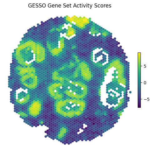
# quickly plot spatial map of activity scores for a specific gene set
figure = gas_report.plot_gas_spatial_map(
geneset="KEGG_PATHWAYS_IN_CANCER", # specify the gene set of interest
size=20, # dot size
cmap="viridis",
figsize=(5, 5),
) # returns a matplotlib Figure object
display(figure)
GESSO (info): Identified 334 common genes in the gene set and expression data.
GESSO (info): Identified 2518 common spots in the location and expression data.
GESSO (info): Normalized expression data with strategy 'normalize-log1p'.
GESSO (info): Model initialization complete.
GESSO (info): Beginning activity score computation for 2 gene sets with 2 jobs. Method
               used: cpu.
GESSO (info): (Job 2:
               WP_INTERACTIONS_BETWEEN_IMMUNE_CELLS_AND_MICRORNAS_IN_TUMOR_MICROENVIRONMENT)
               Activity score computation for
               WP_INTERACTIONS_BETWEEN_IMMUNE_CELLS_AND_MICRORNAS_IN_TUMOR_MICROENVIRONMENT
               completed in 1.09 seconds.
GESSO (info): (Job 1: KEGG_PATHWAYS_IN_CANCER) Activity score computation for
               KEGG_PATHWAYS_IN_CANCER completed in 4.11 seconds.

You can easily retrieve relevant data in pd.DataFrame form from the GESSO gene set activity scores report.
[7]:
display(gas_report.gas_df())
display(gas_report.gene_contributions_df(geneset="KEGG_PATHWAYS_IN_CANCER"))
| KEGG_PATHWAYS_IN_CANCER | WP_INTERACTIONS_BETWEEN_IMMUNE_CELLS_AND_MICRORNAS_IN_TUMOR_MICROENVIRONMENT | |
|---|---|---|
| barcode | ||
| GTAGACAACCGATGAA-1 | -1.137452 | 0.044172 |
| ACAGATTAGGTTAGTG-1 | -0.076933 | -1.285475 |
| TGGTATCGGTCTGTAT-1 | -1.564224 | -1.565298 |
| ATTATCTCGACAGATC-1 | -1.624066 | -0.296113 |
| TGAGATCAAATACTCA-1 | -2.743630 | -0.461900 |
| ... | ... | ... |
| GCCCTGAGGATGGGCT-1 | -3.237531 | 1.022693 |
| CGGGCGATGGATCACG-1 | -2.021051 | -1.913347 |
| TGCGGACTTGACTCCG-1 | -4.610999 | 0.047913 |
| TCGCTGCCAATGCTGT-1 | -3.376165 | 0.271323 |
| GGTGTAGGTAAGTAAA-1 | -1.997408 | 1.049836 |
2518 rows × 2 columns
| KEGG_PATHWAYS_IN_CANCER | |
|---|---|
| ERBB2 | 0.209451 |
| RARA | 0.174657 |
| PRKCA | 0.174332 |
| CDH1 | 0.168812 |
| VEGFA | 0.157994 |
| ... | ... |
| GSTP1 | -0.127424 |
| PDGFRB | -0.139686 |
| CSF1R | -0.144355 |
| FOS | -0.167397 |
| MMP2 | -0.192850 |
315 rows × 1 columns
[8]:
model = GESSO(
    expression_df=expression_df,
    locations_df=locations_df,
    genesets_df=genesets_df,
    k=6,  # increase k to increase spatial smoothing effect
    normalize_counts_method="normalize-log1p",  # easily normalize counts for non-preprocessed data
)
# compute activity scores for all gene sets in genesets_df
gas_report = model.compute_gas(
    beta=0.33,  # increase beta to increase spatial smoothing strength; must be between 0 and 1
    compute_method="cpu",  # either "cpu" or "lowres"
)
# quickly plot spatial map of activity scores for a specific gene set
figure = gas_report.plot_gas_spatial_map(
    geneset="KEGG_PATHWAYS_IN_CANCER",  # specify the gene set of interest
    size=20,  # dot size
    cmap="viridis",
    figsize=(5, 5),
)  # returns a matplotlib Figure object
display(gas_report.gas_df())
display(gas_report.gene_contributions_df(geneset="KEGG_PATHWAYS_IN_CANCER"))
GESSO (info): Identified 334 common genes in the gene set and expression data.
GESSO (info): Identified 2518 common spots in the location and expression data.
GESSO (info): Normalized expression data with strategy 'normalize-log1p'.
GESSO (info): Model initialization complete.
GESSO (info): Beginning activity score computation for 2 gene sets with 2 jobs. Method
               used: cpu.
GESSO (info): (Job 2:
               WP_INTERACTIONS_BETWEEN_IMMUNE_CELLS_AND_MICRORNAS_IN_TUMOR_MICROENVIRONMENT)
               Activity score computation for
               WP_INTERACTIONS_BETWEEN_IMMUNE_CELLS_AND_MICRORNAS_IN_TUMOR_MICROENVIRONMENT
               completed in 1.08 seconds.
GESSO (info): (Job 1: KEGG_PATHWAYS_IN_CANCER) Activity score computation for
               KEGG_PATHWAYS_IN_CANCER completed in 4.11 seconds.
| KEGG_PATHWAYS_IN_CANCER | WP_INTERACTIONS_BETWEEN_IMMUNE_CELLS_AND_MICRORNAS_IN_TUMOR_MICROENVIRONMENT | |
|---|---|---|
| barcode | ||
| GTAGACAACCGATGAA-1 | -1.137452 | 0.044172 |
| ACAGATTAGGTTAGTG-1 | -0.076933 | -1.285475 |
| TGGTATCGGTCTGTAT-1 | -1.564224 | -1.565298 |
| ATTATCTCGACAGATC-1 | -1.624066 | -0.296113 |
| TGAGATCAAATACTCA-1 | -2.743630 | -0.461900 |
| ... | ... | ... |
| GCCCTGAGGATGGGCT-1 | -3.237531 | 1.022693 |
| CGGGCGATGGATCACG-1 | -2.021051 | -1.913347 |
| TGCGGACTTGACTCCG-1 | -4.610999 | 0.047913 |
| TCGCTGCCAATGCTGT-1 | -3.376165 | 0.271323 |
| GGTGTAGGTAAGTAAA-1 | -1.997408 | 1.049836 |
2518 rows × 2 columns
| KEGG_PATHWAYS_IN_CANCER | |
|---|---|
| ERBB2 | 0.209451 |
| RARA | 0.174657 |
| PRKCA | 0.174332 |
| CDH1 | 0.168812 |
| VEGFA | 0.157994 |
| ... | ... |
| GSTP1 | -0.127424 |
| PDGFRB | -0.139686 |
| CSF1R | -0.144355 |
| FOS | -0.167397 |
| MMP2 | -0.192850 |
315 rows × 1 columns
You can also work directly with gene sets in dictionary form.
[9]:
model_alt = GESSO(
    expression_df=expression_df,
    locations_df=locations_df,
    k=6,
    normalize_counts_method="normalize-log1p",
    verbose=False,  # per-call override: suppress all messages from this model
                    # (for finer control, use gesso.logging - see above)
)
gas_report = model_alt.compute_gas(
    genesets_dict=genesets_dict,
    beta=0.33,
    compute_method="cpu"
)
gas_report.plot_gas_spatial_map(
    geneset="KEGG_PATHWAYS_IN_CANCER",
    size=20,
    cmap="viridis",
    figsize=(5, 5)
)
[9]:
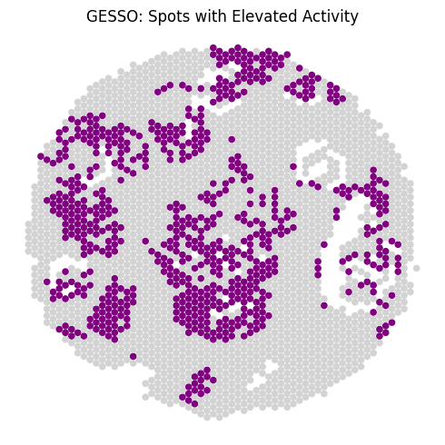
Use GESSO to systematically identify spots with significantly elevated gene set activity
Please note that the output of the permutation-based hypothesis test varies with the total number of genes in the dataset. The example dataset used in this demo contains a subset of all genes from the original dataset.
[10]:
model = GESSO(
    expression_df=expression_df,
    locations_df=locations_df,
    genesets_df=genesets_df,
    k=6,
    normalize_counts_method="normalize-log1p",
    verbose=False
)
htest_report = model.htest_elevated_gas(
    geneset="KEGG_PATHWAYS_IN_CANCER",
    beta=0.33,
    n_permutations=100, # number of random gene sets to sample for the test
    n_jobs=4            # set number of CPUs
)
[11]:
display(htest_report.htest_df())
htest_report.plot_pval_spatial_map(
    size=20,
    significance_threshold=0.05
)
| x | y | gas | p | |
|---|---|---|---|---|
| barcode | ||||
| GTAGACAACCGATGAA-1 | 7 | 55 | -1.137452 | 0.97 |
| ACAGATTAGGTTAGTG-1 | 7 | 57 | -0.076933 | 0.32 |
| TGGTATCGGTCTGTAT-1 | 7 | 59 | -1.564224 | 1.00 |
| ATTATCTCGACAGATC-1 | 7 | 61 | -1.624066 | 1.00 |
| TGAGATCAAATACTCA-1 | 7 | 63 | -2.743630 | 1.00 |
| ... | ... | ... | ... | ... |
| GCCCTGAGGATGGGCT-1 | 68 | 74 | -3.237531 | 0.96 |
| CGGGCGATGGATCACG-1 | 69 | 75 | -2.021051 | 0.98 |
| TGCGGACTTGACTCCG-1 | 68 | 76 | -4.610999 | 0.98 |
| TCGCTGCCAATGCTGT-1 | 68 | 80 | -3.376165 | 0.95 |
| GGTGTAGGTAAGTAAA-1 | 70 | 50 | -1.997408 | 0.93 |
2518 rows × 4 columns
[11]:
[ ]: